Gradient Wars - Reparametrization vs REINFORCE

A ride through gradient estimators

Happy new year 🎉🎇🎆! I was cleaning the dust out of some past handwritten notes on REINFORCE, when I decided to write up this short post, comparing the method against the known reparametrization trick, most often seen in training Variational Autoencoders.

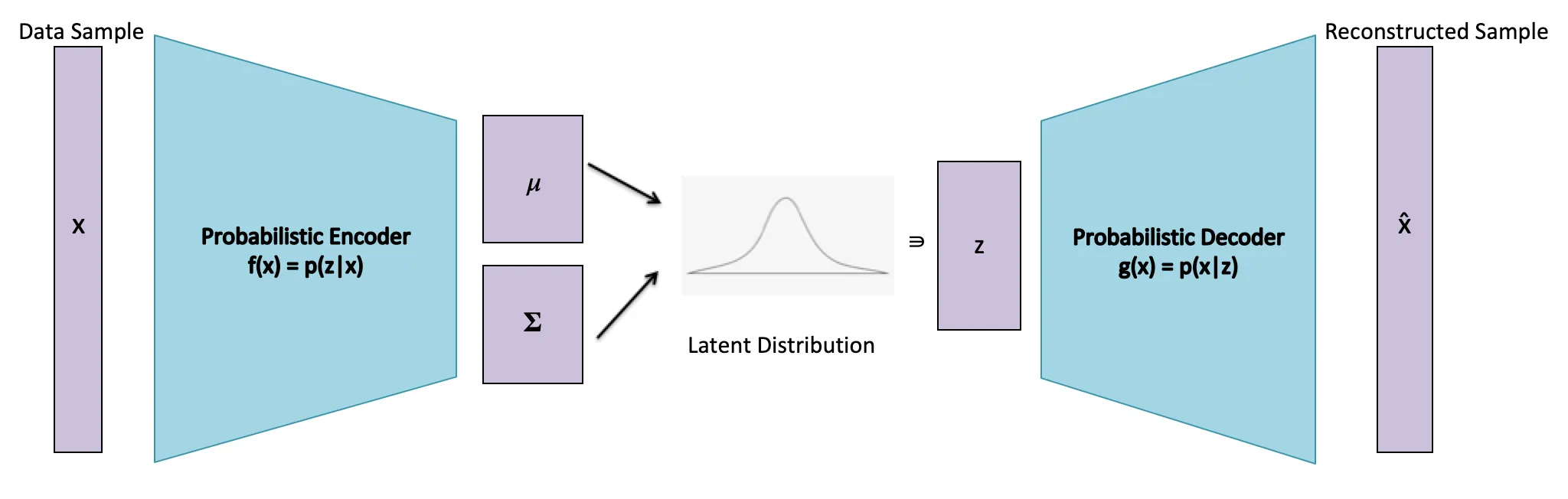
Variational Autoencoders (VAEs), introduced by Kingma and Welling , are a class of deep latent variable models consisting of two coupled, independently parametrized components: an encoder(recognition model) and a decoder (generative model). Without going out of scope with details, the true posterior distribution over the latent variables is intractable to compute directly, so a variational approximation is used instead. A concrete example would be a prior \(p(z)\) as an isotropic Gaussian distribution and the stochastic encoder is modeled as a multivariate normal \(\mathcal{N}(\mu_\theta(z), \text{diag}(\sigma_\phi(z)))\), where \(\mu_\theta(z)\) and \(\sigma_\phi(z)\) are neural networks. The decoder is similarly structured with a neural network mapping the latent variable \(z\) back to the data space, thus enabling efficient learning of both the generative process and the inference model.

As an image is a thousand words, I directly borrow an excellent illustration of a Probabilistic Autoencoder by Elzette van Rensburg, as discussed before.

The Problem

Consider a random variable \(z \sim p_\theta (z)\), where \(p_\theta\) is a parametric distribution and a function \(f\), for which we wish to compute the gradient of its expected value. For instance, \(f\) may express a cost function such as the likelihood. If our aim is to minimize the likelihood \(L(\theta) = \mathbb{E}_{z \sim p_{\theta}(z)}[f(z)]\), or more formally \(\min \left\{ L(\theta) = \mathbb{E}_{Z \sim p_{\theta (z)}} [f(z)] \right\}_\theta\), then we are interested in evaluating (or at least, estimating) the gradient

\[\nabla_\theta \mathbb{E}_{z \sim p_{\theta}(z)}[f(z)]\]

where the variable notation \(z\) is used to refer to computing the expected value from a variable in the latent space. The issue here lies in computing the expectation with respect to the parameter distribution \(p(z)\), making it inherently stochastic instead of deterministic. That’s where path-derivative gradient estimators come to the rescue.

The Reparametrization trick

The reparametrization trick can be briefly expressed as follows: If the distribution is reparameterizable, then \(z = g(\theta, \epsilon)\), where \(g\) is a deterministic function of parameters \(\theta\) and \(\epsilon\) is an independent random variable (noise). This leads to:

\[\frac{\partial}{\partial \theta} \mathbb{E}_{z \sim p_\theta(z)}[f(z)] = \frac{\partial}{\partial \theta} \mathbb{E}_\epsilon [f(g(\theta, \epsilon))]\]

Which simplifies to:

\[\mathbb{E}_{\epsilon \sim p_\epsilon} \left[ \frac{\partial f}{\partial g} \frac{\partial g}{\partial \theta} \right]\]

Thus, \(z\) is reparameterized as a function of \(\epsilon\), and the stochasticity of \(p_\theta\) is pushed to the distribution \(q(\epsilon)\), where \(q\) can be chosen as any random noise distribution. For example, if \(Z \sim N(\mu, \sigma^2)\), then \(z = \mu + \sigma \cdot N(0, 1)\). Another example would be, for a uniformly distributed variable \(U \sim U(a,b)\), that \(u = a + (b - a) \cdot U(0, 1)\).

This bright trick alters the expectation to a distribution independent of \(\theta\), which can now be computed using Monte Carlo estimation, provided that \(f(g_\theta(\epsilon))\) is differentiable with respect to \(\theta\). Assuming a batch sample of size \(N\), the gradient estimator is

\[\nabla_\theta \mathbb{E}_{x \sim p(x)}[f(x)] \approx \frac{1}{N} \sum_{i=1}^{N} \nabla_\theta f(g_\theta(\epsilon_i))\]

The reparametrization trick belongs to the family of Path-derivative gradient estimators. Path-derivative estimators focus on how the expected value of a function changes as a parameter of the underlying distribution changes. This is done by considering a “path” through the parameter space. By expressing the sampled value as a deterministic function of a differentiable random variable, it creates a smooth and differentiable path for the sampling process.

A really intuitive illustration of the above, borrowed from the excellent writing of Kingma and Welling is shown here:

Score function Estimator - REINFORCE

Another gradient estimation method is the score-function estimator (SF) (also known as likelihood-ratio, or more commonly, REINFORCE) , which exploits the log-derivative property. It relies on the score-function (gradient of the log-likelihood) to estimate the gradient, without expressing the random variable as a function of a differentiable random variable (as in path-derivative estimators).

The differentiation rule of the logarithm is \(\nabla_\theta \log p_\theta(z)= \frac{\nabla_\theta p_\theta(z)}{p_\theta(z)} \Rightarrow \nabla_\theta p_\theta(z) = p_\theta(z) \nabla_\theta \log p_\theta(z)\), where \(\nabla_\theta \log p_\theta(z)\) is known as the score-function. Hence we can rewrite the gradient as

\[\nabla_\theta \mathbb{E}_Z [f(z)] = \mathbb{E}_Z \left[ f(z) \nabla_\theta \log p_\theta(z) \right]\]

REINFORCE only requires that \(p_\theta(z)\) is differentiable with respect to the parameters \(\theta\), and it does not require backpropagating through \(f\) at the sample \(z\). It must also be easy to sample from \(p_\theta(z)\). Just like before, for a sample batch of size \(N\), we approximate the expectation as

\[\mathbb{E}_Z \left[ f(z) \nabla_\theta \log p_\theta(z) \right] \approx \frac{1}{N} \sum_{i=1}^{N} f(x_i) \nabla_\theta \log p_\theta(x_i)\]

which is an unbiased estimator of the gradient (in plain terms, for infinite sample size the above expected value is the same as the true gradient). Although unbiased, known drawback of REINFORCE is high variance of the estimation, leading to slow training convergence for relatively small samples. Finally, it is worth noting that the variance of SF can be reduced by substracting a control variate \(b(z)\) as follows:

\[\begin{split} \nabla_\theta \mathbb{E}_Z [f(z)] &= \mathbb{E}_Z [f(z) \nabla_\theta \log p_\theta(z)] \\ &= \mathbb{E}_Z [f(z) \nabla_\theta \log p_\theta(z) + b(z) \nabla_\theta \log p_\theta (z) - b(z) \nabla_\theta \log p_\theta(z)] \\ &= \mathbb{E}_Z [(f(z) - b(z)) \nabla_\theta \log p_\theta (z) ] + \mu_b \end{split}\]

where \(\mu_b \equiv \mathbb{E}_Z [b(z) \nabla_\theta \log p_\theta(z)]\). Known estimators with control variates are NVIL , MuProp (unbiased), VIMCO among others.