Beyond Prediction: Why Causality Matters
And what your ML models are missing
Introduction 🥚🐥
Modern data systems, from recommendation engines to climate analytics, are built almost entirely on predictive modeling. In a nutshell, one collects a vast number of observational samples (that are created under variable experimental scenarios), fits increasingly complex models (from simple regression models to fancy deep neural networks), and optimize for accuracy. Pretty much, classification models are fitted on target variables of interest, and decision policies are taken simply using these models. If $f$ is such a fitted classification model and $X$ a vector of features (e.g. cost of acquiring a customer and manufacturing expenses), then one may fit a predictive model on a variable of interest $y$ (e.g. expected sales) by $y = f(X)$ and then use it for sales prediction by plugging in values of $X$. Beneath the surface however lies a fundamental limitation of predictive models, which becomes crucial whenever we want to answer questions such as:
-
❓ What will happen if I set the price of a product to, let’s say, $5$ euros? Will sales increase?
-
❓ Why did an outcome occur?
-
❓ How do we make decisions that remain valid when conditions change (e.g. we test a drug on mice and are interested whether its effect changes under a distribution shift, e.g. on a population of humans)
Overall, predictive models excel at recognizing associations. Causal models on the other hand represent the underlying mechanisms of data. The difference between the two, although subtle at first, defines the boundary between pattern recognition and scientific reasoning. As Scholkopf et al.
If we wish to incorporate learning algorithms into human decision making, we need to trust that the predictions of the algorithm will remain valid if the experimental conditions are changed.
In this post, we’ll walk through why causal models matter, how causal reasoning differs from prediction and illustrate the stakes, along with a minimal example. It does not serve as a complete treatment of causality, but as a motivational introduction to the unfamiliar reader. For a thorough treatment, we refer the interested reader to
Why Causality Matters
Predictive models rely on observed correlations and patterns in observational data (i.e. samples that are purely observed, not obtained under a specific manipulation of the examined system). They implicitly assume that all samples come from a single, stable distribution (the familiar i.i.d. assumption). Under this assumption, identifying strong associations can be enough to make good and powerful predictions.
However, associations alone cannot tell us what causes what. Consider the following, basic example:
Predicting Ice Cream Sales 🍦
It is known that during the summer, ice cream sales are increased compared to other seasons, with number of sunburn cases also showing an higher trend. We know (taken as expert knowledge) that although these two quantities are correlated, ice cream sales do not cause sunburn cases and vice-versa. Instead, these two quantities share a confounder (common cause) like the sun’s radiation, or even temperature. In any case, even if they have more than one confounding variable, we are allowed to treat them both as a single. The fact that $\text{ice cream sales} \leftarrow sun \rightarrow \text{sunburn}$, highlights our previous discussions, where a directed arrow represents a direct causal relationship (from a cause to its direct effect(s)).
Now imagine an alternate world where everyone wears suncreen 🧴 (we intervened on sun’s radiation indirectly, by forcing lower radiation by sunscreen use): Sunburn cases plummet, but ice cream sales remain unchanged.Will ice cream sales increase, decrease or remain unaffected (similarly for sunburn cases)?
A predictive model would infer: more sunburn → more ice cream sales. We know this is wrong, but the model doesn’t. Both variables are effects of a third, hidden cause: sunlight intensity. This unobserved confounder creates misleading correlations, and as a result, any predictive model trained on the original correlation will catastrophically fail, and any inferred decisions cannot be taken seriously.
This example captures the core limitation of predictive modeling:
💡 Predictive patterns break when the observed environment changes, while causal mechanisms do not.
The following table briefly shows scenarios where predictive and causal queries differ, and as a result, how predictive models can lead to false interpretations.
| Task | Query | Example | Description | Causal Model | Predictive Model |
|---|---|---|---|---|---|
| Prediction | Predict / diagnose $Y$ given $X$ | “What is $Y$ when $X_1$ = 5?” | Standard supervised prediction | ✔️ Correct predictions | ✔️ Correct predictions |
| Decision Making | Optimal $X$ to increase $Y$ under constraints | “What $X_1$ maximizes Y given $X_2 = 6$?” | Choosing an action that changes the system | ✔️ Correct decisions | ❌ Possibly wrong decisions |
| What-if | Hypothetical changes (interventions) | “What if I set $X_1 = 5$?” | Interventional reasoning, requires $do(X)$ | ✔️ Correct estimate | ❌ Possibly wrong estimate |
| Interpretation | Feature importance / effect of $X$ on $Y$ | “Does $X_1$ affect $Y$?” | Understanding influence of features | ✔️ Correct estimate | ❌ SHAP/feature importance may be misleading |
| Counterfactual | “What would $Y$ have been if $X$ had been different?” | “$Y=3$ when $X_3=$yellow. What if $X_3$=green?” | Individual-level alternative-world reasoning | ✔️ Correct estimate | ❌ Generally impossible |
| Root Cause | Identify cause of an event | “What caused the failure?” | Find initial causal driver | ✔️ Correct estimate | ❌ Possibly wrong |
The Common Cause Principle
But how can observational data mislead us? Reichenbach’s common cause principle
💡 If X and Y are correlated, then either X causes Y, Y causes X, or a hidden confounder causes both.
Observational data cannot tell these apart. This limitation explains famous phenomena like Simpson’s paradox
Randomized Experiments: The Gold Standard for Causality
Given the limitations of observational data, a natural question arises: how can causal effects be measured correctly? Since the seminal work of Ronald Fisher
Randomized experiments aim to isolate causal effects by deliberately intervening on one or more variables of interest while holding all other factors constant in expectation. This is typically achieved through random assignment, which ensures that both observed and unobserved covariates are, on average, balanced across experimental groups. As a result, randomization removes confounding by design, allowing causal effects to be identified without relying on strong modeling assumptions.

Common instances of randomized experimentation include:
- Randomized Controlled Trials (RCTs) in medicine and the social sciences,
- A/B tests in online platforms and digital systems,
- Controlled laboratory experiments in the natural sciences,
- Simulation-based interventions in synthetic or virtual environments.
To illustrate, consider a clinical trial investigating whether a newly introduced treatment (let’s call it $X$) reduces the severity of migraines. An RCT proceeds by randomly assigning patients to either a treatment group (receiving treatment X) or a control group (receiving a placebo), and subsequently comparing outcomes across the two groups. Because assignment is random, any systematic difference in outcomes can be attributed to the intervention itself rather than to pre-existing differences among patients.
A standard causal quantity estimated in such settings is the Average Treatment Effect (ATE), defined as $\text{ATE} = \mathbb{E}[Y_1 - Y_0]$ where $Y_1$ and $Y_0$ denote the potential outcomes under treatment and control, respectively. If the ATE is statistically distinguishable from zero, one concludes that the intervention has a causal effect on the outcome of interest.
The conceptual strength of RCTs lies in their ability to eliminate confounding bias through randomization, making them the most reliable tool for causal inference. However, despite their methodological appeal, randomized experiments are often impractical or infeasible in real-world settings. They can be prohibitively expensive, logistically complex, or ethically unacceptable, for instance, when studying the causal effects of harmful behaviors such as smoking. Moreover, in modern large-scale systems, the space of possible interventions is often combinatorial, rendering exhaustive experimentation impossible in practice.
These limitations motivate the development of model-based causal frameworks that allow causal effects to be inferred without relying exclusively on randomized experiments. In the following sections, we introduce such a framework through structural causal models, which enable principled reasoning about interventions, counterfactuals, and distributional changes beyond purely observational data.
The Language of Causality - SCMs & Pearl’s Ladder
The formal language in Causality to reason about causal mechanisms, interventions and counterfactuals are Structural causal models (SCMs), introduced by Judea Pearl
- A Directed Acyclic Graph (DAG) where nodes represent the examined variables of interest and direct arrows direct causal effects (e.g., Sun → IceCream).
- Structural equations ($X_i = f_i(\mathrm{Parents}(X_i), \epsilon_{X_i})$), representing how each variable $X_i$ is generated.
- Independent noise terms $\epsilon_{X_i}$ for each variable $X_i$, representing unobserved and inherent randomness of the system.
This framework allows us to compute three fundamentally different types of queries:
| Type | Question | Example |
|---|---|---|
| Observational | What do we see? | $P(Y \mid X=x)$ |
| Interventional | What happens if we force X to a value? | $P(Y \mid do(X=x))$ |
| Counterfactual | What would have happened otherwise? | $P(Y_{x’} \mid X=x,Y=y)$ |
Predictive models only answer the first type, while causality accounts for all three.
SCMs allow us to simulate interventions mathematically without performing physical experiments. Using do-calculus, we can compute $P(Y \mid do(X=x))$ which differs from the purely observational $P(Y \mid X=x)$ except in special, unconfounded cases (outside the scope of this blog). This gives us a way to predict interventions, if we know the causal graph.
How Do We Discover Causal Graphs?
This is where the field of causal discovery enters. Causal discovery attempts to learn the structure of the system (the DAG) from data (often observational, sometimes including interventional samples), which operate under certain causal assumptions. For example, the causal sufficiency assumption assumes no hidden confounders, while faithfulness (loosely defined in the scope of this blog post) that no determinism exists in the examined system, hence no causality (e.g. variables that are deterministically related like ratios of variables). Once the graph is known, causal inference methods estimate effects such as:
- ATEs
- mediation effects
- optimal intervention strategies
- counterfactual outcomes
In practice, as the ground truth causal model is unknown, one first discovers the causal structure (the causal DAG and the SCM representation) and then estimates causal effects.
An Illustrative Example The provided examples are available in a curated Github Repository (https://github.com/kougioulis/causality-tutorial) with various causality tutorials for the motivated reader.
Consider 3 variables, $X,Y,Z$. $X$ and $Z$ are observed to have correlation coefficient $3$. That is, if you observe $1$ unit of change in $X$, you observe $3$ units of change in $Z$. Let’s try to answer the following questions:
- ❓ If you intervene and change $X$ (not merely observe) in the real world, what change would you observe?
- ❓ If you build a predictive model from $X$ to $Z$ and change the input to the model, would you observe the same change when you intervene in the real world?
For linear correlations and causal relations with Gaussian additive noise, we make the following assumptions:
- ☝️ Correlations on a path multiply together
- ☝️ Correlations from different path sum
We begin by importing some needed modules:
import numpy as np
import pandas as pd
import statsmodels.api as sm
import matplotlib.pyplot as plt

np.random.seed(42)
Consider a causal DAG, assuming linear relationships with edges $X \leftarrow Y \rightarrow Z$ and $X \rightarrow Z$. A directed edge illustrates direct causal influence (i.e. $X$ directly causes $Y$, $X$ is the direct cause of $Y$, $Y$ is the direct effect of $X$) while indirect causal relationships are illustrated by directed paths. The linear coefficients of each causal edge are $0.7$ for $Y \rightarrow X$, $-8$ for $Y \rightarrow Z$ and $13$ for $X \rightarrow Z$. Loosely defined, pairing this causal DAG with the functional dependencies of its variable given its parents (direct causes), plus an additive noise term (accounting for randomness), creates an (additive) structural causal model (SCM). Let’s try to answer the following question:
What is going to happen when I increase X by 1?
- The non-causal path $X \leftarrow Y \rightarrow Z$ has coefficient $0.7 \cdot (-8)=-5.6$.
- The path $X -> Z$ coefficient $13$ causal effect causal path.
- The total correlation coefficient observed is $0.7 - 8 = -7.3$.
We observe that the causal effect is larger than the computed correlation! (Causal effect is positive, observed correlation is negative)
We define the SCM of the three variables:
# Defining structural equations of the SCM
# X <- Y (coef 5) + noise
# Z <- Y (coef -2) + X (coef 13) + noise

n_samples = 10**6  # large enough sample size

# Exogenous Gaussian noise
eps_y = np.random.normal(0, 1, n_samples)
eps_x = np.random.normal(0, 1, n_samples)
eps_z = np.random.normal(0, 1, n_samples)

# Structural Causal Model
Y = eps_y
X = 0.7 * Y + eps_x
Z = -8 * Y + 13 * X + eps_z

data = pd.DataFrame({"X": X, "Y": Y, "Z": Z})
And compute the observed Pearson correlation between X and Z, as well as the predictive effect (regression $Z \sim X$):
# Pearson Correlation between X and Z (observational / predictive)
corr_xz = np.corrcoef(X, Z)[0, 1]

# Predictive model: Z ~ X by ordinary least squares regression
X_df = sm.add_constant(data["X"])
model_pred = sm.OLS(data["Z"], X_df).fit()
pred_effect = model_pred.params["X"]

print("Observed correlation between X and Z:", round(corr_xz, 3)) # 0.862
print("Predictive effect (regression Z ~ X):", round(pred_effect, 3)) # 9.246
From the above snippet, we obtain the following contradictory results:
-
Causal model: Increase $X$ by $1$, increase Z by $0.86$.
-
Predictive model: Increase $X$ by $1$, increase Z by $9.25$.
The correct approach, would instead be to:
- 1️⃣ Learn the causal model (via a causal discovery algorithm, in this example we assume it is known correctly.)
- 2️⃣ Identify the non-causal paths and remove the effect of the non-causal paths and only (identify the quantities that block the correlations from non-causal paths, called the adjustment set).
- 3️⃣ Build a predictive model that includes an adjustment set and only and hence controls for their values.
The correlation coefficient of $X$ to $Z$ conditioned on fixed values of $Y$ provide the true causal effect of $13$ units with the following code snippet, with an absolute error in the third decimal place.
# True causal effect (by an intervention do(X))
causal_effect = 13  # known from our structural equations

# Adjustment set approach (control for Y in regression)
XZ_df = sm.add_constant(data[["X", "Y"]])
model_adj = sm.OLS(data["Z"], XZ_df).fit()
adj_effect = model_adj.params["X"]

print(f"Causal effect (true do-intervention): {causal_effect}") # 13
print(f"Causal effect via adjustment set (regression Z ~ X + Y): {round(adj_effect, 3)}") # 13.002

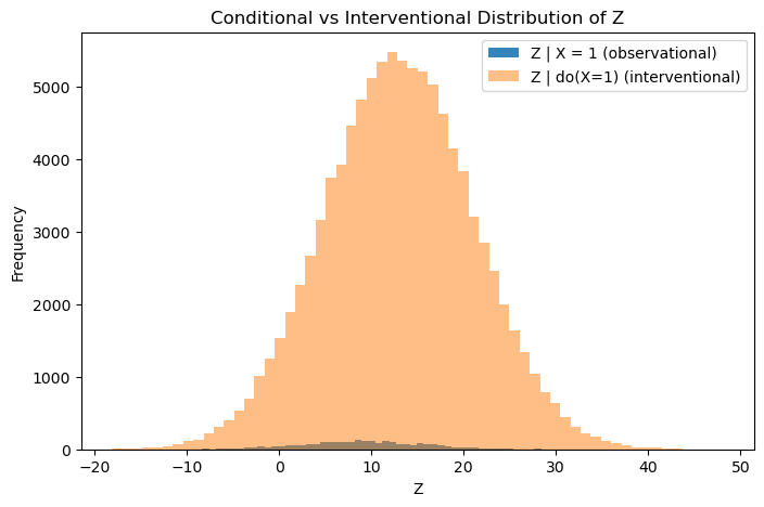
As shown in the histogram, the two distributions $Z \mid X \approx 1$ and $Z \mid do(X = 1)$ differ dramatically because:
-
Under conditioning, when we observe $X = 1$, that typically means Y was high, because $X = 0.7Y + \text{noise}$. Thus the backdoor path $X \leftarrow Y \rightarrow Z$ pushes Z down via the $-8Y$ term.
-
Under intervention, when we force $X = 1$, $Y$ is no longer correlated, so only the direct causal effect $(13X)$ applies.
Back to the Ice Cream Sales Example
Let’s return to the ice cream example illustrated at the beginning of the post, but this time with some code:
from sklearn.linear_model import LinearRegression
import numpy as np
import matplotlib.pyplot as plt

np.random.seed(42)
samples = 500  # observational samples (iid)

# True causal mechanism: ice_cream sales <- sun -> sunburn
sun = np.random.uniform(0, 10, size=samples)
ice_cream = 2 * sun + np.random.normal(0, 1, size=samples)
sunburn = 3 * sun + np.random.normal(0, 1, size=samples)

# Predictive model incorrectly learns sunburn -> ice cream
X = sunburn.reshape(-1, 1)
pred_model = LinearRegression().fit(X, ice_cream)

# Intervene: sunscreen campaign sets sunburn to a constant
sunburn_intervened = 3 * np.ones(samples)

# Predictive model's WRONG prediction under intervention
predicted_icecream = pred_model.predict(sunburn_intervened.reshape(-1, 1))

# True causal outcome under intervention - ice cream depends ONLY on sunlight, not sunburn (graph surgery is performed on the underlying SCM)
true_icecream = 2 * sun + np.random.normal(0, 1, size=samples)

print(f'True Ice Cream Sales (causal model): {true_icecream.mean():.2f} units') # 10.04 units
print(f'Predicted Ice Cream Sales (predictive model): {predicted_icecream.mean():.2f} units') # 2.05 units
A predictive model wrongly suggests that an increase in one unit of radiation will account for two units of increase in ice cream sales, which is 5 times less that the true causal effect which we obtained using the true causal model.
As we have noticed already, a predictive model is doomed to failure if applied to cases outside the trained distribution: For example, consider applying the above simple regression model on a hypothetical subpopulation of Scandinavians (who are less exposed to sunlight compared to other regions) who enjoy eating ice cream all year long.
Closing Thoughts
Predictive models excel at finding patterns in data, but patterns alone are not enough when decisions, interventions, or changing environments are involved. Predictive models (either from classical ML up to deep learning approaches) have found great sucess, yet they prove unstable when the underlying perturbed.

Causal modeling addresses this gap by explicitly representing how data is generated. By reasoning about interventions and counterfactuals, causal methods allow models to generalize beyond the conditions under which they were trained and to support meaningful actions.
It is to no surpise that decades after Pearl’s formulation of causality, the industry is just starting to adopt causal discovery and causal inference methods for optimized decision making and creation of causal digital twins, especially in the case of time-series data (by Temporal Structural Equation Models - TSCMs
What’s your view? Let me know in the comments! 🚀
If you found this post useful, please cite this as:
Kougioulis, Nikolas (Dec 2025). Beyond Prediction: Why Causality Matters. https://nkougioulis.com.
or as a BibTeX entry:
@article{kougioulis2025beyond-prediction-why-causality-matters,
  title   = {Beyond Prediction: Why Causality Matters},
  author  = {Kougioulis, Nikolas},
  year    = {2025},
  month   = {Dec},
  url     = {https://nkougioulis.com/blog/2025/causal-predictive/}
}
